The advertisements on this site are selected by me, and represent content that I believe is high quality or interesting. Purchasing content from these links helps me get paid as a content creator.

Flow Matching for Generative Modeling (Paper Explained) - Yannic Kilcher

Yannic Kilcher Summary

Understanding Diffusion Models | 0:00:00-0:06:00
Defining an Approximate Distribution with a Gaussian Mixture Model | 0:06:00-0:19:20
Connecting Flow with Probability Density Path | 0:19:20-0:30:00
Conditional Flow Matching for Neural Networks | 0:30:20-0:40:20
Optimal Transport Path vs. Diffusion | 0:40:20-0:46:20
Stable Diffusion 3 and Recap | 0:46:20-0:52:40

Understanding Diffusion Models | 0:00:00-0:06:00

https://youtu.be/7NNxK3CqaDk?t=0

Hello there! Today, we're delving into generative models, focusing on flow matching as presented by researchers from Meta.ai and the Weizmann Institute of Science. This topic is more technical but fundamental to understand the evolution of diffusion models. Interestingly, "Stable Diffusion 3," deviates from classic diffusion-based approaches, transitioning to this more general flow matching technique.

FLOW MATCHING FOR GENERATIVE MODELING (arxiv.org)

We examined this paper, along with "Stable Diffusion 3," during our Saturday night discussions on Discord. If you're interested in joining us, we host them nearly every Saturday; they're always fascinating. The insights I'll share are largely contributed by the community, so kudos and thanks to them. Discord: https://ykilcher.com/discord

Usually, diffusion models are applied for image generation, notably text-to-image generation. Consider DALI, where you input a prompt such as "dog in a hat," and the output is an image to match that description. The image generation process in this context is typically a diffusion process.

Importantly, this method varies from traditional GAN or VAE image generation approaches, as a diffusion process is a multi-step procedure that can invest more computational power in generating an individual image than simply performing a singular forward pass.

A diffusion process initiates with an image comprised entirely of random noise derived from a standard Gaussian distribution. Throughout the process, intermediate computations gradually de-noise the picture until the final target image is achieved. The model training method consists of using an image from the dataset, incrementally enhancing its noisiness.

If performed correctly and sufficiently, regardless of the initial image, the concluding distribution would be a standard normal distribution. The key is to continuously add noise until the original signal is completely obliterated, resulting in a known final state distribution. Consequently, it's possible to sample from this distribution and, by learning to reverse each intermediary phase, trace back these steps to reconstruct something akin to the original data.

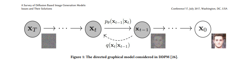
A Survey of Diffusion Based Image Generation Models: Issues and Their Solutions (arxiv.org)

So a diffusion process starts with a data set, continuously adds noise, so there is a noising process in order to construct a series of intermediate data points, so this is t equals 1, t equals 2, and so on until t equals infinity, and you learn a neural network to revert one of those steps. So this here could be neural network V at t equals 2 reverting one noising step. So it looks at a noisy image and produces a slightly less noisy image.

Once you possess the neural network, you can reverse the denoising steps. There are numerous advances, tips, and tricks in diffusion models that allow you to bypass certain stages, rather than proceeding step by step. Modern diffusion methods, in fact, directly try to forecast the final state, then add noise to create a less noisy version, and predict the final state again. This is an ongoing process, but the fundamental principle is to define a denoising process, and then attempt to reverse it.

Defining an Approximate Distribution with a Gaussian Mixture Model | 0:06:00-0:19:20

https://youtu.be/7NNxK3CqaDk?t=400

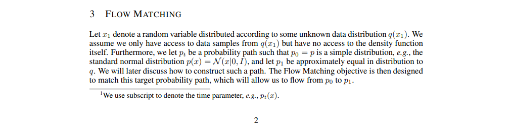
Flow matching expands on this concept, questioning the necessity of defining a fixed denoising process and the issues related to it. Instead, it suggests starting with a probability distribution, one-dimensional for the sake of this explanation.

Clearly, there are several problems. The foremost is that we don't know the distribution; we have no clue what it is. What we can do, however, is define an approximate distribution using the samples we have. Let's assume we have three data samples. We can construct a pseudo distribution using some sort of Gaussian mixture model. A Gaussian mixture model places a Gaussian at each data point, integrates over them, and gives a distribution. We call this approximate target distribution Q, which is purely defined by the data.

What if we learn how to morph the standard initial distribution p0 into Q? That's what flow matching is about how to construct this transformation from one distribution to a second one, having only samples available from the second distribution. One key component is going to be the efficient morphing of one sample into another. This process is known as conditional flows.

Through a series of proofs, it can be shown that managing this transformation using single samples is sufficient to characterize the entire flow between the two distributions. This mathematical contribution shows that we only need to worry about single paths, like single samples, and aggregating them will give the correct probability distribution.

The paper also deals with practical aspects, like how to implement this in a feasible way which we can compute.

You might wonder what differentiates diffusion at the top, where we defined the noising process explicitly, and flow matching at the bottom. Flow matching is a more comprehensive approach. If you define flows in a certain manner, you can recover the diffusion process.

The paper defines a probability density path. This function, being time-dependent, is known as a probability density path. Input consists of our data distribution (Rd) and a time variable ranging from 0 to 1.

To illustrate, imagine a 2D data space with an initial Gaussian distribution around zero. We want to transform this into a different data distribution, say a Gaussian centered around a different point with a smaller standard deviation.

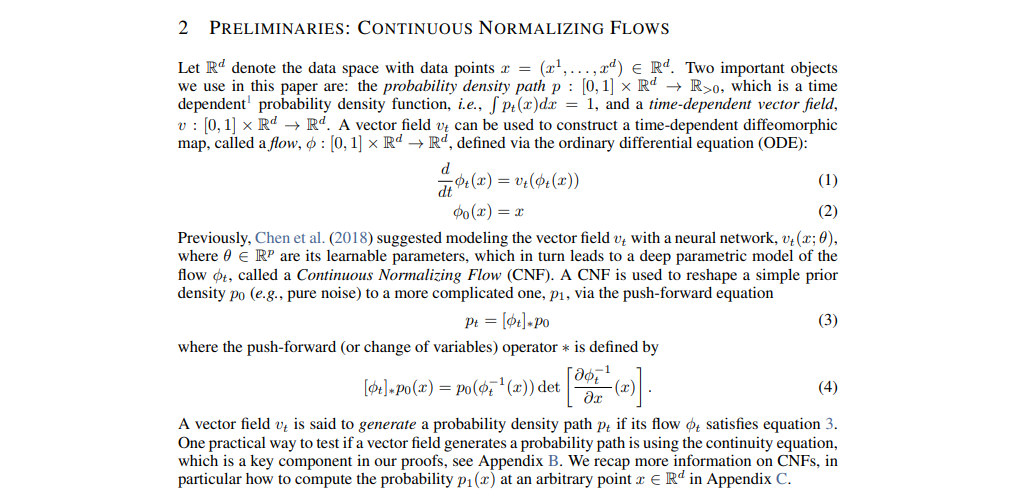
Another key concept is a time-dependent vector field, denoted as V. V differs in that it requires both a time and location to navigate to Rd. This concept is tied to the next object, termed a time-dependent diffeomorphic map or flow, which is linked to the vector field in a specific way. What does this mean? It means that the flow at time 0, of any point, is simply that point.

In lay terms, consider the flow at time 0 to be the point itself, with the flow's change defined by the vector field.
V will determine the flow of each point at a particular time, serving as the instantaneous rate of change a speed, if you will.
If a point were at a location, it would move to a position as dictated by the vector field, always aimed towards a predetermined distribution.
As V determines the direction and speed of a point's move, any point following V over time will eventually land in a corresponding position within the resulting set.

The probability density paths haven't been connected yet, but the vector field already designates a mode of movement. By following the vector field, the end position will be at t equals 1. The aim is to construct a vector field capable of processing the data distribution we originally had, e.g., this Gaussian. If each point in this distribution follows the vector field, they will reach the target probability distribution.

The vector field's time-dependent nature is crucial. It evolves, not staying fixed. Initially, at t equals 0, it sets a direction. However, this direction may change over time, leading to a constantly shifting vector field. This ongoing change defines the 'flow,' showing how each point moves over time according to the vector field's momentary direction.

Practically, the result often simplifies into a constant vector field that aligns with optimal transport goals, making implementation easier. Yet, the vector field can remain time-dependent, requiring careful management. To use this effectively, we begin by sampling a starting point, like from a Gaussian distribution. Then, we apply an ODE solver to guide the process continuously until t equals 1. Once we have this time-dependent vector field, we can proceed with the procedure.

Our primary focus is understanding and learning about this time-dependent vector field, as it defines the flow's characteristics and guides our approach to distribution transformations.

Connecting Flow with Probability Density Path | 0:19:20-0:30:00

https://youtu.be/7NNxK3CqaDk?t=1160

Now, let's discuss the definition of the flow, which involves setting the vector field to generate a probability density path under the condition that the flow adheres to equation three. This is how we connect a flow with the probability density path. Essentially, we push the original probability density through the flow, which is just a way of moving. If we take the density and push it through the flow, we end up with the probability density path. This ensures that every point in the density moves along with the flow.

Imagine taking each point, each with its corresponding density value, moving these through the flow. This results in a different density, hopefully the target density. What do we do next? We regress that flow, meaning the construction.

This seems deceptively simple. Essentially we take a neural network, v, along with this probability density path and the vector field generating it. Then we regress that, learning to match this vector field for each position and time.

This sounds straightforward, but the challenging part is figuring out the probability density paths and the corresponding vector fields. This is where the paper's contribution comes in. As we stated before, we may not know the probability density of the target distribution, but we can approximate it with samples. We can do this with a Gaussian mixture model at the target samples.

We can also generalize this by defining the probability density path and vector field in terms of individual samples. In this section, they discuss constructing a target probability path from a mixture of simpler paths given a particular sample x1. This is denoted as a conditional probability path based on one particular sample of data. Here, the 1 signifies it's at time t equals 1, or part of the actual data distribution at the end of the process. It explores how our probability flow would look if we condition it on that particular sample.

Boundary conditions are defined such that at time 0, the probability density should just be the density of our original source distribution. Say, if we sample from a standard Gaussian, no matter what the target data point is, at time 0 we're in this plain, data-independent source distribution. At time t equals 1, we can design p1 to be a distribution concentrated around the data point. This can be done through a Gaussian with the mean at the data point and a small standard deviation, resulting in a small Gaussian centered at that data point. They discuss marginalizing the conditional probability paths over the target data, which gives rise to the marginal probability path.

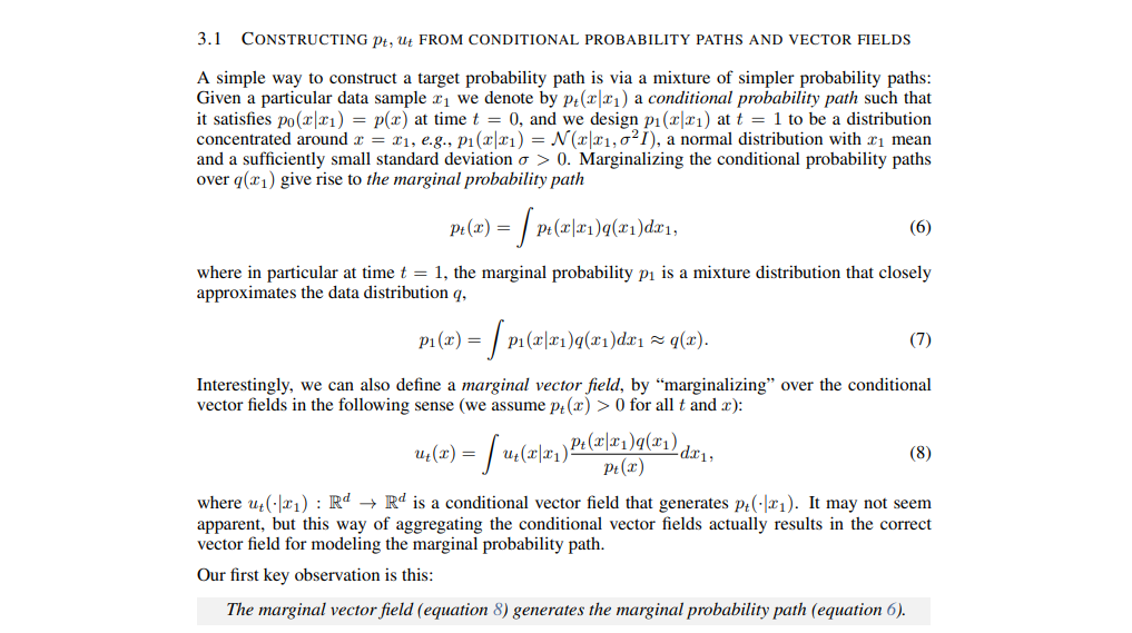
The question becomes how to aggregate the individual data points. The answer is to marginalize them, considering all the target data and aggregating across them, yielding a total probability path. From the individual sample paths, we can create a whole probability path. This path closely approximates the data distribution at time t equals 1.

Interestingly, they also define a marginal vector field by marginalizing over the conditional vector fields. Given that we can figure out what the vector field is for an individual sample, we need to know if we can aggregate these across samples and create a total vector field. This is possible, as long as we weigh them by a specific factor. This total vector field can be made from the individual vector fields. We know these factors have been figured out, and we can create a Gaussian mixture distribution of the target data as long as we reweigh by them.

A key observation is that the marginal vector field generates the marginal probability path. They demonstrate that if we define the vector field this way, it will generate this probability path. If we push the source distribution along the vector field over time, it will end up at the target distribution by following this probability path.

This may not seem significant, but it connects how to move individual samples between source and target and how to transfer the entire distribution from source to target. That's one of the main recognitions, and what will make it feasible to action this because we can only operate on samples; we cannot perform extensive integrations across full distributions.

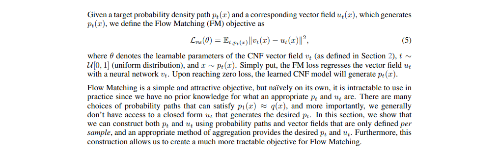
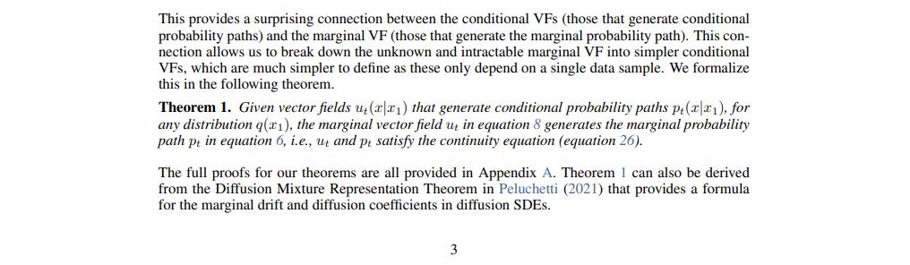
Due to intractable integrals in the definitions of the marginal probability path and the vector field, it remains unachievable to calculate 'u' and therefore, to naively compute an unbiased estimator of the original flow matching objective. Instead, we suggest a simpler objective, which, surprisingly, will yield the same optima as the original objective: the conditional flow matching objective. So, what's next?

Conditional Flow Matching for Neural Networks | 0:30:20-0:40:20

https://youtu.be/7NNxK3CqaDk?t=1820

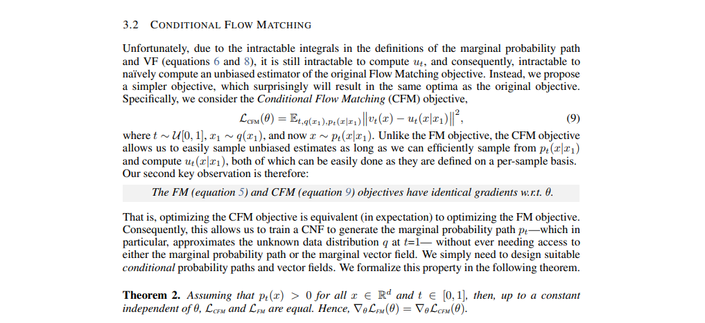
Rather than calculating the entire vector field, we can aggregate this from individual samples. This removes the need to perform the full integration process; instead, we request the neural network to learn this from the data. This is still intractable, but we can perform the same trick as before, employing conditional flow matching. This allows us to perform flow matching on individual samples.

We sample a target data point and a source data point, which also involves sampling a probability path. While we don't know how these paths are constructed, essentially, we sample a path from a point in the source distribution going to the target distribution. As long as we can regress on the vector field rising from this sample along this path, we're fine. This has the same gradients as the original flow matching loss. Thus, flow matching and conditional flow matching losses are equal. So, the neural network parameters are identical.

We don't need to first aggregate and train a neural network to predict the entire vector field. Instead, we can have the neural network predict the conditional vector field based on an individual data point. Achieving this results in the same parameters as our initial goal if we learn optimally. Further, the paper's structure seems odd, as it first proposes what to learn assuming we can perform the tasks and later explains how to get the probability path.

The paper advances the theory in a general-to-specific manner, with the authors making specific choices for practicality or tractability. They propose constructing the probability paths using a series of normal distributions to interpolate between the original and target distributions. Intermediate distributions thus will resemble Gaussian distributions, with time-dependent functions defining the mean and standard deviations. The authors have chosen an isotropic Gaussian distribution, which may align linearly or non-linearly with the diffusion objective.

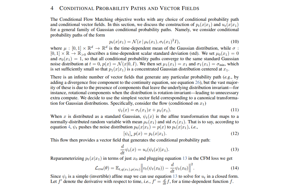
The approach now focuses on using Gaussian distributions deliberately. At t equals zero, the goal is to match the original distribution, while at t equals one, the shift is towards centering the Gaussian around the data point with a smaller standard deviation, leading to the desired Q target distributions as data accumulates.

The transition process is straightforward, involving scaling the original data point by sigma and adjusting the mean. This defines a push forward and outlines its evolution over time. However, this process is essentially a mathematical interpretation of following the trajectory and scaling it based on the corresponding standard deviation.

This simplifies the calculation for the flow matching loss, where a Gaussian probability path is defined along with its corresponding flow map. This map follows the trajectory dictated by mu t and sigma t, maintaining its Gaussian form. The vector field, crucial to this path, is determined by the derivatives of the mean and standard deviation functions, linking back to Gaussian processes.

Importantly, these functions are not defined at their boundaries. In relation to diffusion, it was previously stated that the noise distribution is achieved when t equals infinity. To reach the actual noise distribution, one must endure the noise until t equals infinity. This distinction is crucial for flow matching, where defining paths that reach the target distribution within a finite period is possible.

Optimal Transport Path vs. Diffusion | 0:40:20-0:46:20

https://youtu.be/7NNxK3CqaDk?t=2420

Interestingly, this divergence can be seen when making specific choices for the Gaussian paths. The Gaussian paths cannot compute the end (say, at t equals one) because t equals one in the flow-matching framework corresponds to t equals infinity in the diffusion framework or vice versa. However, a more straightforward proposal is to move linearly. This path, referred to as the optimal transport path, indicates that the vector field's direction remains constant and always points to the target distribution. At every point in time, this vector field suggests moving towards the target.

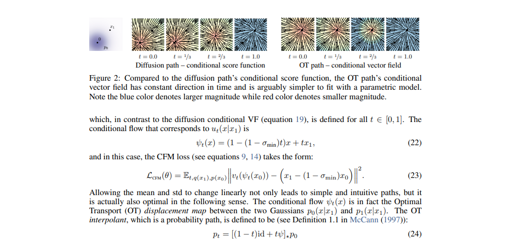
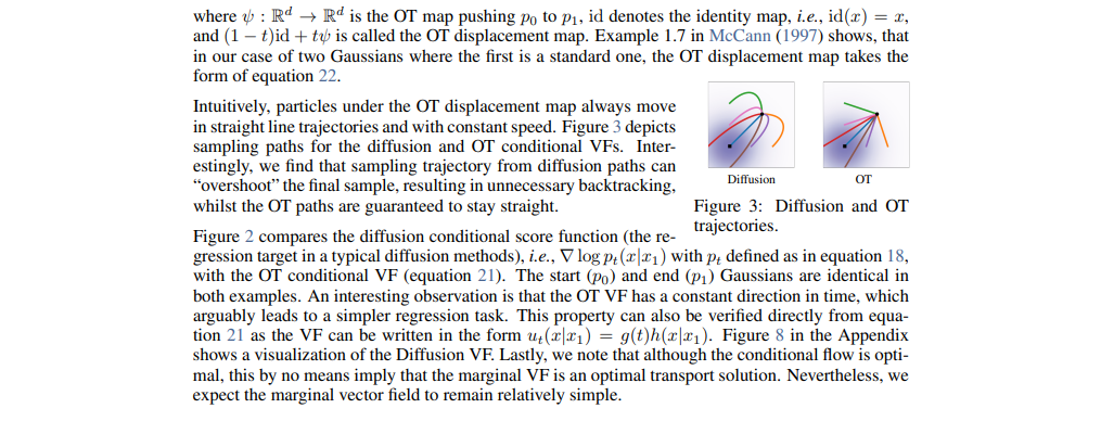
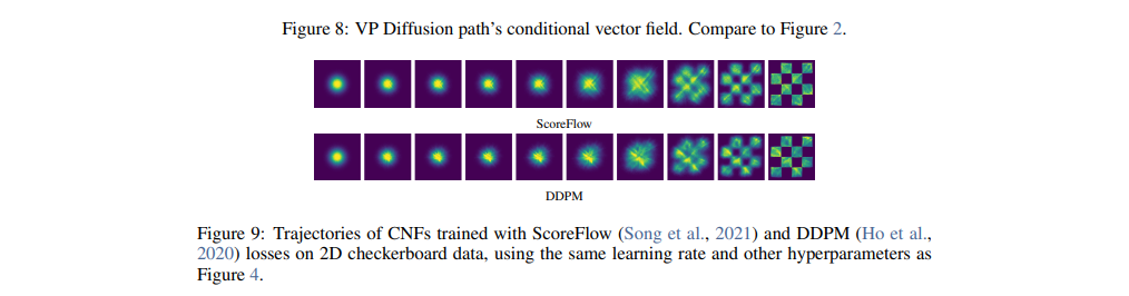
In comparison, the diffusion path, driven by a score function rather than directly regressing the vector field, behaves differently, at a particular point, it will push points ahead and eventually curve back to the target. The reason lies in the data generation process, where noise is added to a data point, causing an external movement before moving towards the target, leading to unique curve shapes in the reverse process.

Therefore, they are not going to end up at the true n distribution. That's why the comparison with the conditional vector field in the appendix, corresponding to this score function, is illuminating. This illustration highlights how the source distribution is pushed, pulled around the target point, and then finally drawn into the intended target.

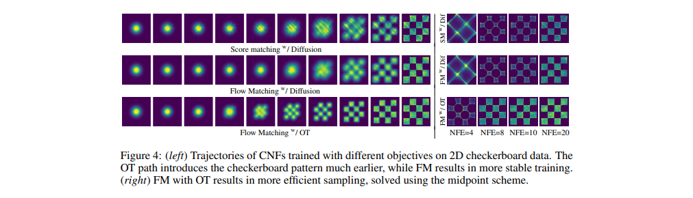
Examining how a sampling procedure works further clarifies the differences. In the experimental section, it becomes evident that the optimal transport objective shapes the target distribution much earlier, while the diffusion objective, whether score matching or flow matching, shapes it much later. Notably, the optimal transport objective requires fewer function evaluations. The implementation approach involves using an ODE solver to push a data point forward through the learned vector field. It's demonstrated that this can be done more efficiently using the optimal transport objective compared to the diffusion objective. This comparison between the diffusion and optimal transport trajectories deepens our understanding of these two techniques.

Stable Diffusion 3: Sampling Time Steps and Paths for Training | 0:46:20-0:52:40

https://youtu.be/7NNxK3CqaDk?t=2780

Stable Diffusion 3 uses a more detailed system to sample these time steps during training, pinpointing the optimal paths and techniques to scale operations. The fundamentals are established here.

Diffusion takes a dataset and delineates a noise process, thereby locking itself into a unique method of denoising and morphing the probability distribution. Conversely, Flow Matchings retracts one step and instead defines vector fields from data to effect flows from source to target. It discovers how to instruct any point in space on the directions to follow to the target, without considering the process that necessitated it.

Assuming we can generate this from existing data, we could then train a neural network to propose iterations for undiscerned data. This method would call for a sample from the source distribution to maneuver along the vector field, as indicated by the neural network. If executed correctly, it would reveal an accurate point in the target distribution.

The simplest and most theoretically sound method is to establish straight lines in the data space between a source and a target sample and base predictions on that the target distribution learned from each straight line defined by a data sample.

Upon opting for optimal transport, essentially a direct path between the source and target sample, we can define the loss. The path or vector field is characterized by a flow. For a given sample, we take x1 and x, and we move linearly toward it. This interpolation, scaled by the standard deviation, helps identify the loss.

We train the vector field to match itself to a derivative of the flow at a certain point. This predictor learns to consider the weightage of the direction distribution. The vector field predictor, with all data sets' aggregation, constructs an entire flow representation.

Consequently, it learns to point each point in space towards the entirety of the data set. Simply applying the derivative to the flow quantity will help us achieve this. The vector field predictor will flow the entire source distribution to the entire target distribution.

Flow Matching for Generative Modeling (Paper Explained)

Affiliate Marketing