Mamba: Linear-Time Sequence Modeling with Selective State Spaces (Paper Explained) - Yannic Kilcher

Yannic Kilcher Summary

Table of Contents

1. Mamba Linear Time Sequence Modeling with Selective State Spaces | 0:00:00-0:09:20
2. Introduction to Mumba Architecture and Selective State Spaces | 0:09:20-0:20:20
3. Overview of Mamba Architecture Components | 0:20:20-0:21:20

Mamba Linear Time Sequence Modeling with Selective State Spaces | 0:00:00 - 0:09:20

https://youtu.be/9dSkvxS2EB0?t=0

Mamba is considered a potential competitor to Transformers, boasting superior scaling properties. I'm curious as to how it differs from existing technologies such as Transformers, Recurrent Neural Networks (RNNs), and state-space models like S4.

There are always interesting trade-offs among these options. Within the context of Transformers, if you deal with a sequence of information, attention allows each piece to interact with any other. With causal attention, for example, when examining a certain input, it allows us to selectively consider another input and integrate it into the computation of the next layer. Thus, a Transformer can dynamically and selectively consider individual elements of the past and address each one separately. However, there is a drawback to this approach. If L represents the sequence length, the model necessitates L-squared computation and potentially L-squared memory requisites, posing a challenge.

On the other hand, RNNs, when confronting a sequence, can only look back one time step in computing the next layer, and even then, it doesn't consider the most recent input. The procedure involves calculating a hidden state for each input by updating a current consideration with the current input. This consideration updates in sequence with each input, taking into account only the last hidden state and the current input to determine the next hidden state. This method allows for the processing of infinitely long inputs with minimal memory requirements. In a system with L computations, you compute as many elements as there are. The memory requirements are determined by the size of the hidden state, inputs, and outputs.

However, problems arise when backpropagation is introduced. Primarily, it requires the remembrance of the entire sequence of intermediate values for back propagation purposes. RNNs utilize a method known as backpropagation through time.

This entails computing the hidden state from the last hidden state and the current input, and then the next hidden state, and ultimately leading to an output.

To adjust a particular transition because there is some type of loss, requires backpropagation through all computations involved in generating hidden states from each other. And because there are numerous time steps to override, this can usually be either prohibitively memory-consuming or can lead to vanishing or exploding gradient problems due to numerous operations, often multiplicative.

Solutions to such issues include long short-term memory (LSTMs) networks that incorporate built-in gating mechanisms. It should be noted that a function determines the next hidden state, and this function generally can be anything.

This paper goes on to discuss the S4 type of state space models. These models have several commendable properties, including functioning like an RNN while simultaneously computing all outputs in one step when given a sequence of inputs, thanks to the formulation of the computation as a convolution operator. This efficiency stems from two factors: 1) the transition from one hidden state to the next is purely linear with no non-linearities, and 2) the backpropagation through time features linear computations up until it diverges into individual elements.

A purely linear operation without any non-linearities is more tractable in terms of gradient complications. This approach facilitates smoother computation and hopping to any point in the process. Absence of dependence on time or input keeps state transitions consistent. The matrices involved are independent of the input, which allows for the pre-calculation of aggregation. The total computation can thus be accomplished as one large operation by multiplying individual inputs from time steps.

Introduction to Mumba Architecture and Selective State Spaces | 0:09:20 - 0:20:20

https://youtu.be/9dSkvxS2EB0?t=560

The question is, where does Mamba fit in? Mamba is an architecture that utilizes selective state spaces, a concept that relaxes a certain property of S4. Specifically, it slightly adjusts the idea that transitions from step to step are independent of input, nudging S4 closer to LSTMs. However, Mamba retains the property of being computable in one swoop, similar to a prefix sum or a parallel scan. Consequently, its training phase resembles a transformer model where whole sequence forward passes are calculated all at once. However, its inference stage is more similar to LSTMs. For such scenarios, possessing a lengthy context and utilizing it efficiently outweighs the benefit of transformers, which is chiefly their ability to focus intensely on individual states.

Structured state-space models were created to compete with transformer models' computational efficiency over long sequences. However, they have not delivered comparable results with transformer models for several significant modalities like language. A critical weakness these models exhibit is their inability to execute context-based reasoning.

In response to this weakness, the researchers propose a new selective state-based model which enhances prior work on several fronts. The goal was to achieve the modeling power of transformers while enjoying linear scalability in sequence length. They identified a key limitation of preceding models to be their inefficiency in selecting data dependent on input.

In structured state space models, you have a prior hidden state, a current input, and a future hidden state (t plus 1). These models usually employ a parameterized function, represented as A, and something different, represented as B. The resultant formula looks something like HT plus 1 equal to A HT plus B X. In such a model, A and B are fixed for the duration of the sequence.

This system is very different from transformers where A, the attention matrix, is dynamically built during each forward pass. Here, every token generates queries, keys, and values, which makes the construction of the hidden state highly dependent on the input, preceding state, and other variables. By contrast, in a structured state space model, everything is fixed, making it even more restrictive than LSTMs.

In an LSTM, signal propagation is determined by the prior hidden state and input, setting it apart from state space models and general recurrent neural networks. Mamba introduces a method where transitions hinge on the present input, not the previously hidden state. This feature permits the pre-calculation of the transition matrix A throughout time. In Mamba, A and B are shaped by the input but not the past hidden state, creating a compromise between state space models and recurrent neural networks. To overcome computational issues, Mamba uses an algorithm attuned to the hardware that calculates the model recurrently with a scan, not a convolution. This approach bypasses the necessity for time and input invariance in prior structured state space models for the sake of efficiency.

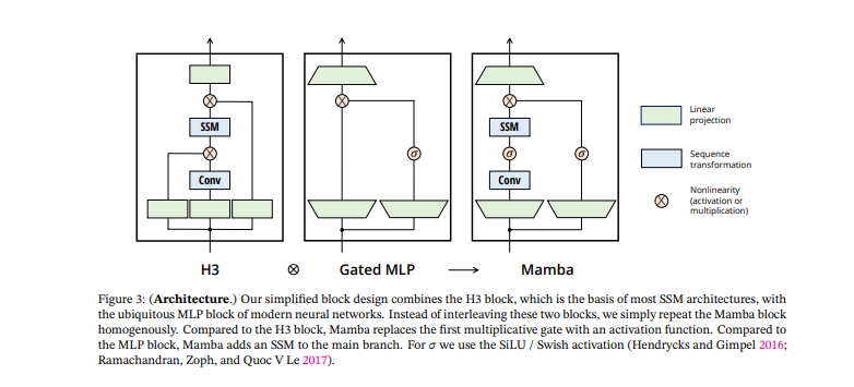
Mamba that employs GPU acceleration to expedite computation, despite using a different algorithm. Mamba integrates Selective State Spaces, 1D convolutions, up-projection, as well as gating to form the Mamba architecture. This design is attention-free.

Fully recurrent models with key attributes such as selectivity could outperform attention-based models like transformers in dense modalities such as language and genomics. Selectivity is significant in boosting performance by introducing a data-dependent transition through hidden states. While the scalability of models like S4 may not suit language tasks, maybe incorporating selectivity could increase performance. The full impact of these advancements, however, remains to be seen.

In order to match the performance of transformers, a transition that is dependent on a hidden state, similar to LSTMs, is necessary. However, the model's capacity may rival transformers in key benchmarks due to its sole dependence on input data. The model offers quick training and inference, linear memory scaling with sequence length, and efficient auto-repetition during inference without the necessity for a key-value cache. It requires only the memory of the last hidden state and involves straightforward matrix multiplications to generate additional tokens. Further, the model operates without attention mechanisms, making it effective for long context scenarios, and demonstrates performance improvements on real data with sequence lengths up to one million.

Overview of Mamba Architecture Components | 0:20:20 - 0:21:20

https://youtu.be/9dSkvxS2EB0?t=1220

The Mamba architecture also includes other components. You would need to envision these components layered atop one another, where the entire sequence is always taken into account during training. Take this for instance; here is a linear projection where dimensions are being projected upwards, projecting each token separately, as in a transformer, followed by a 1D convolution and the presence of some non-linearity, and finally comes the SSM.

In these two processes, you would want to consider the entire sequence as one while training. Whereas in these projections, to the best of my understanding, they individually handle tokens similar to the MLPs present in a transformer.

The architecture contains a gating mechanism positioned between layers and not time steps, along with residual connections. The Mamba architecture introduces a selective state space layer equipped with a time direction designated for calculating tokens in a sequence. This process involves accumulating hidden states over time during both training and inference. The backbone of this process involves multiplication and modulation using an A matrix and input to produce the next hidden state within the state space structure.

Discretization in state space models which were initially designed for continuous time systems. Their conversion to discrete time requires a different approach to maintain accuracy. Despite the criticality of discretization, understanding deep learning and data flow perspectives often ignore it.

There are four parameters in the context of matrices or vectors with learnable parameters. They control the amount of input that is being propagated into the new hidden state and how the hidden state is processed into the output state. You can see the next hidden state is generated from the previous hidden state, multiplied by what is termed A-bar. A-bar is simply a computation that results from this discretization parameter and the A matrix. Don't fret over it; consider, if you wish, that this here is a learnable matrix and this here is another learnable matrix. Looking at this from a higher perspective, one could see that this is a very simple, plain recurrent neural network without any sort of non-linearity around here. You can regard this as just a linear recurrent neural network, where you are just kind of damping in some way, in some multi-dimensional way, the previous hidden state, and then add a projected version of the input. The output is once again calculated as a linear function of the hidden state.

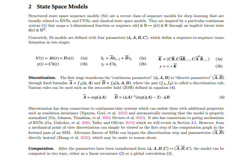
In the scenario of parameter A being fixed, other variables such as B, C, and delta are calculated from the input, thereby leading to input dependency for the zoom function. This subsequently results in an increase in dimensionality for each time step, thereby making the computations L times larger. To address this issue, the GPU balances high bandwidth memory and SRAM (which is faster but smaller memory). SRAM is used for swift matrix multiplications by reducing the need to shift data between different types of memory. By directly loading parameters to the speedy SRAM, carrying out computations, and writing outputs back, time is saved and efficiency improved. They utilize the reduction of data movement and the re-computation of intermediate states to meet similar memory requirements as an optimized transformer implementation. They implement a selective scan layer using a prefix sum technique to handle zoom operations with variable elements, resulting in improved performance. Pre-computing prefix sums to efficiently calculate sums or multiplications in algorithms. By pre-computing the sums or products, one can avoid having to re-compute them while easily calculating the desired values by subtracting or adding pre-computed results. This method proves useful in various algorithms to hasten computations and enhance performance.

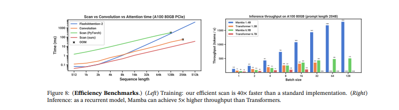
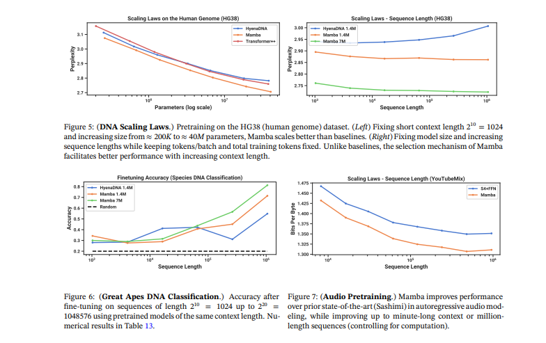
Mamba outperforms all other attention-free models and is the first to match the performance of a very powerful 'transformer plus plus recipe' that has now become the norm, particularly as the sequence length increases. So, the jury is still out on what may occur at significantly large scales, but this already looks promising even at this scale. Mamba trumps other models in DNA modeling because the strength of these types of models truly lies in their long sequence lengths.

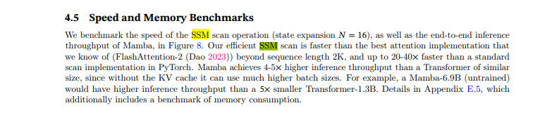
Yet again, it will be interesting to see what the exact trade-off is going to be, whether we need to make the transitions input dependent or not. You can clearly see that the inference throughput on an A100 is impressive and actually becomes more drastic as the batch size increases, especially when you compare it to transformers.

In conclusion, Mamba is a strong contender to become a general sequence model backbone. Lastly, I would like to invite anyone interested to delve deeper into this subject. Look into the efficient implementation intricacies as they discuss or the code here on GitHub. Especially MambaSimple.py, which I recommend you check out first. In fact, the same thing is implemented multiple times in this codebase. One time for Python, one time for GPU, and then another time for inference where you perform things recurrently and once more for training where you compute everything all at the same time.

mamba/mamba_ssm/modules/mamba_simple.py at main · state-spaces/mamba · GitHub

As a result, you will find the same code written in many different ways multiple times. It is worth looking at this step function here because it gives a good idea. The process involves initial input projection, followed by a 1D convolution. Then the parameters for DT are introduced, which then project down and up to put it through a dimensionality bottleneck. The A matrix is a parameter that is stored as log A and not A itself. Discretization in this architecture involves multiplying DT with both A and B, followed by the computation of recurrence using the state times DA plus X. This is how the primary recurrence for the hidden state is determined. The output is gained by multiplying the hidden state by C. There is also a gating connection in D, which is evident in the architecture diagram. This includes projections, 1D convolution, some non-linearity, state space models involving discretization and recurrence computation, a gating pathway involving D matrix, and output projection. This architecture, known as Mamba, provides insights into its functionality and applications and paves the way for exciting advancements in the field.