V-JEPA: Revisiting Feature Prediction for Learning Visual Representations from Video (Explained) - Yannic Kilcher

Yannic Kilcher Summary

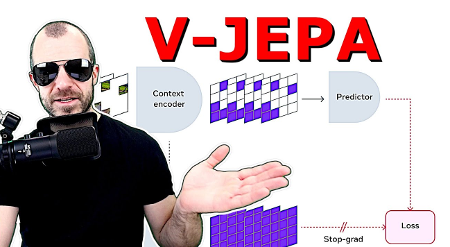
Table of Contents

1. Revisiting Feature Prediction for Learning Visual Representations from Video: The VGEPA Model | 0:00:00-0:01:05
2. Understanding Video through Predictive Feature Principle | 0:01:05-0:07:00
3. Efficiency of vJEPA Compared to Pixel-Based Methods | 0:07:00-0:08:00
4. The Original JEPA Paper | 0:09:20-0:27:05
5. Visual Representation Learning in VGEPA Paper | 0:27:05-0:30:20
6. Predicting Latent Features in Videos | 0:30:20-0:42:00
7. Results and Evaluation | 0:42:00-10:10:10 *

Revisiting Feature Prediction for Learning Visual Representations from Video: The VGEPA Model | 0:00:00-0:01:05

https://youtu.be/7UkJPwz_N_0?t=0

This paper "Revisiting Feature Prediction for Learning Visual Representations from Video", focusing on the V-GEPA model. V-GEPA is a variant of the GEPA architecture by Yann LeCun, based on the concept of feature prediction for unsupervised learning. The model aims to learn latent features from video data to enhance downstream tasks like video classification. Pre-training with VGEPA can improve tasks such as topic classification and feature extraction. This of this model like Bert but for video, in a way, but also very different.

Understanding Video through Predictive Feature Principle | 0:01:05-0:07:00

https://youtu.be/7UkJPwz_N_0?t=65

I want to examine the paper's abstract before proceeding to the original JEPA paper. They assert that humans have an impressive capability to transform low-level signals from the retina into a semantic spatial-temporal understanding of the world. This includes recognizing objects and global motion, all derived from various localized pixel movements. Matching this ability to understand video, specifically, streaming image data, with machines is an extremely challenging feat. A long-standing objective of the machine learning community is to determine the principles or objectives guiding this unsupervised learning in humans.

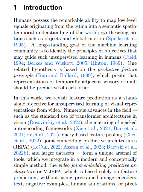
The question poses, how do humans achieve this? How do humans extract high-level constructs from pixel movement? And how do humans learn to do this? Certainly, one could contend that we have an innate ability to do some of this, but we need to learn all the objects that exist in the world, many of which have not existed for all of evolution. Therefore a mechanism must exist for humans to acquire this knowledge unsupervised.

The hypothesis they follow here is the so-called predictive feature principle, which stipulates that representations of temporally adjacent sensory stimuli should predict each other. In layman's terms, we deal with representations, not the signals themselves. This is our first hint that we are not operating in pixel space. Any abstraction from the pixel space will take place in the latent space, and as such, there wouldn't be any pixel reconstruction error or auto-regressive data synthesis.

All activities here occur in the latent space, temporally adjacent sensory stimuli, are video frames that follow one another. We should be able to predict one from another, not the video itself, but its representation. So, if I see an incomplete dog, I can predict that the other half of the dog is likely to appear in the remaining part of the video. Or if I see a road early in the video, I might predict that a car will appear on the road towards the video's end.

The hypothesis proposes that humans learn to extract meaningful features from video data in an unsupervised manner. This is based on the principle that humans associate and predict video representations with each other.

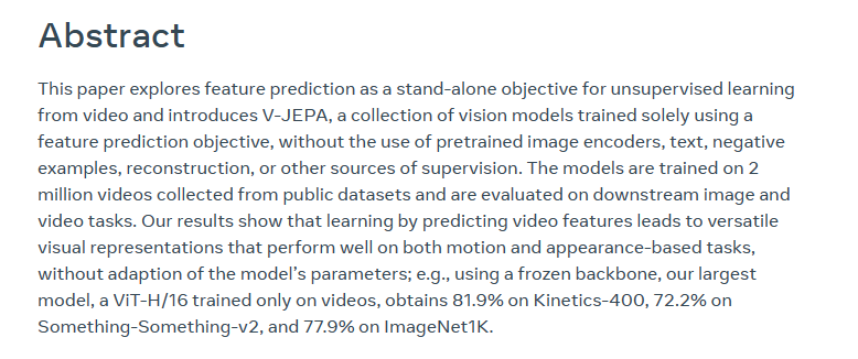
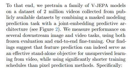
The goal of revisiting feature prediction as a standalone objective for unsupervised learning of visual representations from video isn't to develop the best model. Instead, it's to assess how far we can go with unsupervised learning of representations based on feature prediction. The developers present a video joint embedding architecture, V-JEPA, based solely on feature prediction. This architecture doesn't require pre-trained image encoders, text, negative examples, human annotations, or pixel-level reconstructions, which eliminates certain necessities. For instance, negative examples are often needed in unsupervised representation learning. The learning process usually involves drawing two similar sentences closer while pushing a dissimilar sentence further away. Determining how far to push the dissimilar sentence can prove problematic, leading to the need for hard negatives examples that are similar but not identical but that should be separated.

Efficiency of vJEPA Compared to Pixel-Based Methods | 0:07:00-0:08:00

https://youtu.be/7UkJPwz_N_0?t=420

Pre-trained encoders obviously also help, they also don't want to use that. Human annotations are very costly. And pixel level reconstruction, as we will see, the theme here of this paper is that the method here, V-JEPA, is going to be much more efficient at reaching certain goals than pixel based methods. So it's not that pixel based methods don't work, it's just that they seem to waste a lot of computation, a lot of parameters and so on at doing just a local pixel level stuff so they can really get those pixels right. VJEPA just doesn't care about the pixels, it purely operates in the latent space and therefore can denote devote a much more extensive budget let's say to getting those latent features correct.

The Original JEPA Paper | 0:09:20-0:27:05

https://youtu.be/7UkJPwz_N_0?t=560

https://arxiv.org/pdf/2301.08243.pdf

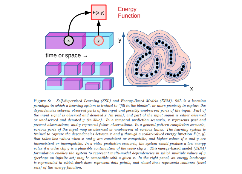
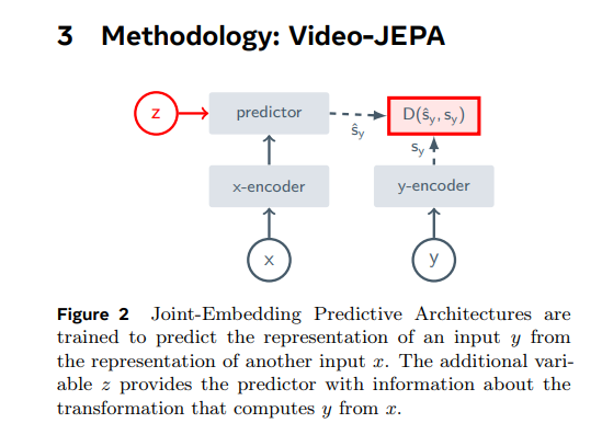
Here is the basic architecture of JEPA, and there are going to be several diagrams. The basic principle is as follows: can we design systems that can take a data point, like a frame from a video or a piece of text, and extrapolate or predict the other part? Or to rephrase, can we design systems that have something called an energy function that can determine whether or not two things go together? For instance, let's imagine a video; if the system knows the beginning, can it predict the continuation?

Even for one start of a video, there are infinite possibilities of continuations. Most of them, as you'd expect, would just be random pixel noise. But among the plausible, natural-looking videos, only some of them would make sense, only some would be valid or probable continuations.

Let's consider an example where a car is driving down a road. Valid continuations could involve the car continuing down the same path, or turning left or right. An invalid continuation would be, for instance, a Disney character suddenly appearing in the next frame. Our aim is to build systems that can recognize whether two parts of data points are a good match. This is what we refer to as the energy function.

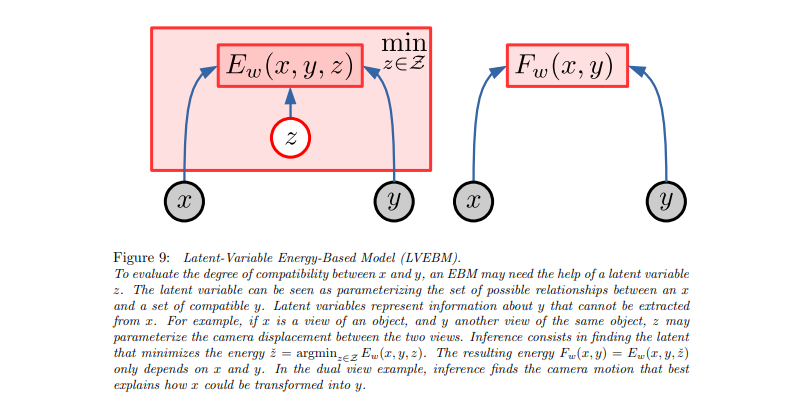
We can extrapolate this principle to a variety of scenarios, all involving hiding some part of the data and attempting to predict it from other parts. To formalize this, we introduce 'z', a latent variable that encapsulates how 'x' and 'y' are interrelated. For instance, in the car example, if we assume three valid paths (left, straight, right), 'z' could encapsulate the choice of direction.

When training these systems, it's crucial to account for the diversity of outcomes for a given 'x'. For instance, if two videos start in the same way but diverge, one showing the car turning left, one showing it turning right, the system shouldn't simply blur the possibilities. The loss should be distinct for each choice and not a blend of all possible outcomes.

In unsupervised feature learning, the challenge is establishing a robust learning process. For instance, learning text embeddings involves deriving a similarity function from a mass of textual data. We often use positive and negative examples to prevent quick collapse, but the paper's authors aim to avoid using negative examples.

The issue with using only positive examples in feature learning is the potential for the system to learn to always output the same results, effectively collapsing the learning process. Therefore, the paper explores ways to prevent collapse in this domain of unsupervised feature learning without relying on negative examples. The authors discuss various methods typically used to prevent collapse and analyze their strengths and weaknesses.

The architecture being discussed serves as a stepping stone towards JEPA. It involves two separate data entities, x and y, which must be connected. The process involves encoding x to create a representation, ultimately leading to the construction of an encoder.

Our ultimate goal, after all training has been completed, is to extract a certain part of it. So it's crucial that we constantly consider what each specific training entails for the encoder. Here we have x, we encode x which gives us S of x, the latent representation, and then we attempt to directly predict y. For instance, I provide the beginning of a video, encode it, and from the latent representation, you give me the pixels for the continuation of the video. I then compare that with the actual pixels and apply my loss function. Although this is similar to an autoencoder, it's not exactly the same; it works from the beginning to the end of the video, predicting outcomes. But, it spends a lot of time and effort on accurately determining the pixels, and it doesn't have the ability to account for a video that could continue in multiple valid directions. The loss itself assumes that there's only one correct outcome. So if I have two different data samples with the same beginning but different continuations, that's seen as noise. Consequently, I would generally opt for taking the mean, as it would incur the least amount of loss. Despite these weaknesses, this method always predicts the pixels, which means my loss back-propagation will always be directed to the encoder, resulting in a satisfactory encoding.

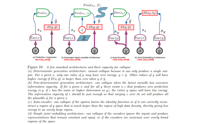
Moving on to the generative latent variable architecture, it accounts for choices or the fact that the same video can lead to different endings. We use the variable z to encapsulate that uncertainty. The encoder now provides a representation, and the part predicting from the encoding of X, the pixels of Y, now also has that choice. However, this strategy can collapse because the model can decide to put all information in Z and no information in S of X. This results in only predicting y from z and never predicting from S of X, causing the encoder not to receive a good gradient hence a potential collapse.

The autoencoder can also collapse by outputting a static outcome. The joint embedding architecture is particularly prone to collapsing because it abandons predicting pixels. This approach tries to predict features of Y from features of X, which attempts to solve the problem of energy waste in pixel prediction. However, it also runs the risk of constantly outputting a constant vector, rendering the model's loss trivially small without learning a useful representation.

The idea of predicting the latent features is beneficial. If we can predict S of Y from S of X, it means we are fulfilling the hypothesis, demonstrating that our representations are good. However, these representations also need to be informative about data and not collapse into nothingness; otherwise, the prediction is easy but meaningless.

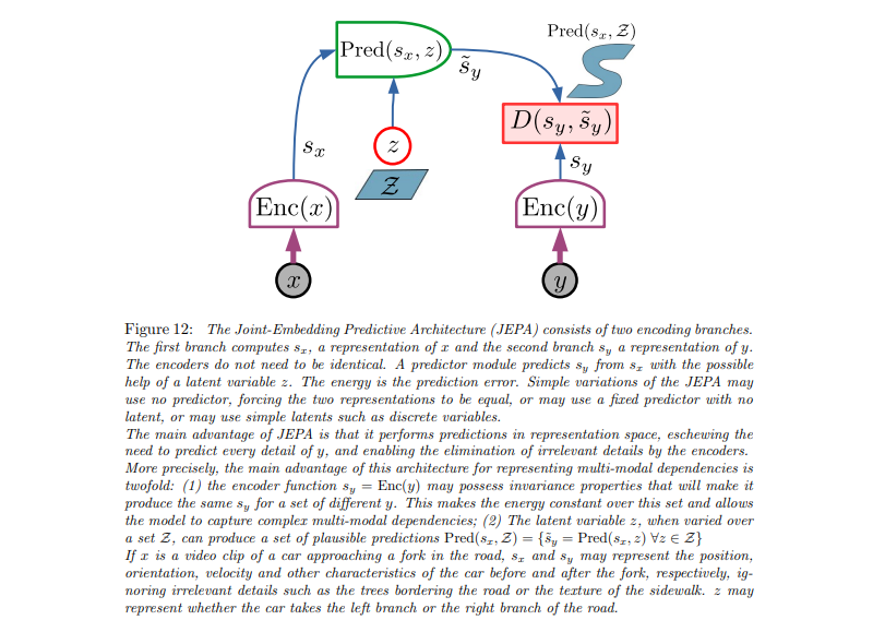
Therefore, the final architecture is designed to incorporate all of these elements. We will have an encoder that provides representation and a choice variable that feeds into the predictor. The predictor then predicts the latent representation of y, followed by a distance metric.

There will be two modifications. First, instead of training this using backpropagation, this will actually be a moving average of the encoder. This method has been successful in other studies where negatives for representation learning like Bootstrap, your own latent, etc., are not used. In this method, we have two encoders, one for x and one for y, but the y train is just a moving average of the weight of x.

The process ensures that the encoding is slightly different from x but still valid. This balance enables the predictor to make sense of the encoding while preventing it from outputting a constant value. The goal is to keep the encoding different enough to avoid easy predictions. The gradient flow only goes one-way due to the moving average, with the trained encoder on the left and constructed encoder on the right. With appropriate timing and hyperparameters, we can achieve collapse while maintaining quality representation learning. If needed, regularizers can be applied for additional optimization. Notably you can slap a regularizer on z to minimize information content, you can slap regularizers on x and y and so on, and there are various derivatives of this, some of which are mentioned in this paper like regularizing covariance matrices on and so on to make things more regular.

Visual Representation Learning in VGEPA Paper | 0:27:05-0:30:20

https://youtu.be/7UkJPwz_N_0?t=1625

Let's now delve deep into the VGEPA paper. As mentioned earlier, the outcome will be the confirmation that feature prediction can, in fact, serve as an effective stand-alone objective for unsupervised learning from video. It achieves this using significantly shorter training schedules than pixel prediction methods. This will result in a versatile visual representation, suggesting we get a model that can input a video and output features that can be utilized for downstream tasks, or fine-tuned for such tasks. It surpasses pixel prediction approaches if it registers better numbers in terms of downstream task operations, or if it equates the downstream task numbers while being quicker to train and more label efficient. So, if there are some labels, it also surpasses pixel-based methods in label efficiency.

Now let's look at the base architecture. For that, we have X and Y, which are two distinct parts of the same video. A common approach is to black out a significant part of the video for the video's entire duration. Then, the prediction is made based on the remaining parts, not based on the pixels, but on the pixel representations. Here, the predictor gets the encoding of X plus the choice variable Z. During training, the Z variable needs to be manually constructed. Hence, we need to define the relation between X and Y manually. They denoted this as delta Y, which is simply the position of the target.

In video processing, blacking out certain parts of the frame impacts delta Y positions. When these parts are run through an encoder, an encoded signal is generated. This encoded information aids in more accurate prediction of the obscured areas based on their relation to the visible content. The encoded data serves as a video frame's representation, functioning as 'Z'. However, this representation is not perfect as it might not account for all future video continuations. The task of creating a flawless 'Z' that considers all variations is quite challenging. If achieving a perfect 'Z' representation is impossible, alternatives such as training-time optimization or learning methods might be necessary.

Predicting Latent Features in Videos | 0:30:20-0:42:00

https://youtu.be/7UkJPwz_N_0?t=1820

This method provides a way for the predictor to utilize visible information to anticipate the representation of unseen elements. Instead of the actual pixels, it predicts the latent features of the video's masked portions.

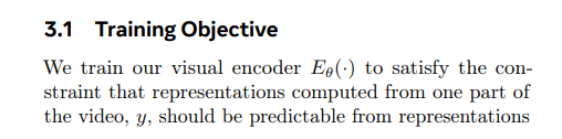
As seen here, our goal is to minimize an L1 loss, and we'll encode X and then predict Y's encoded features. We'll apply an L1 loss over this and subsequently jointly train the predictor and the embedder more effectively. To avert a collapse, we'll implement some modifications: adding a stop gradient in the y direction and incorporating a moving average. We'll structure the y encoder to be a moving average of the x encoder. The decision to apply an L1 regression was simply to ensure greater stability.

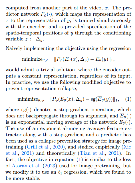
The motivating factor behind this adaptation of an exponential moving average, consolidated from another paper, principally boils down to the supposition that if the optimal predictor is assumed, then the encoder's gradient can be computed - which is the significant factor because if there is a collapse, the encoder's gradient would be data-independent, implying the encoder is data-independent and during the training, the encoder's gradient becoming data-independent would be anticipated. However, under certain suppositions, they can compute that gradient in a closed form, which demonstrably contains the data, thus making it data reliant.

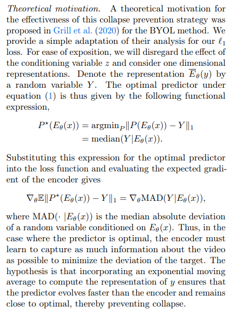
This indicates that the encoder learns from the data and avoids a collapse. Inclusion of an exponential moving average to calculate the y representation ensures the predictor evolves faster than the encoder and stays close to optimal, thereby preventing collapse.

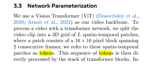
Although this is merely a justification and not proof, it is acceptable as is. This will form the basis of the V-JEPA architecture. Let's start on the left hand side. The video will be divided into patches; in this context, tokens will be synonymous with patches. These patches will measure 16 by 16 pixels, encompassing two sequential frames of that size, hence creating volumes of pixels (admittedly, this is quite a poor volume.

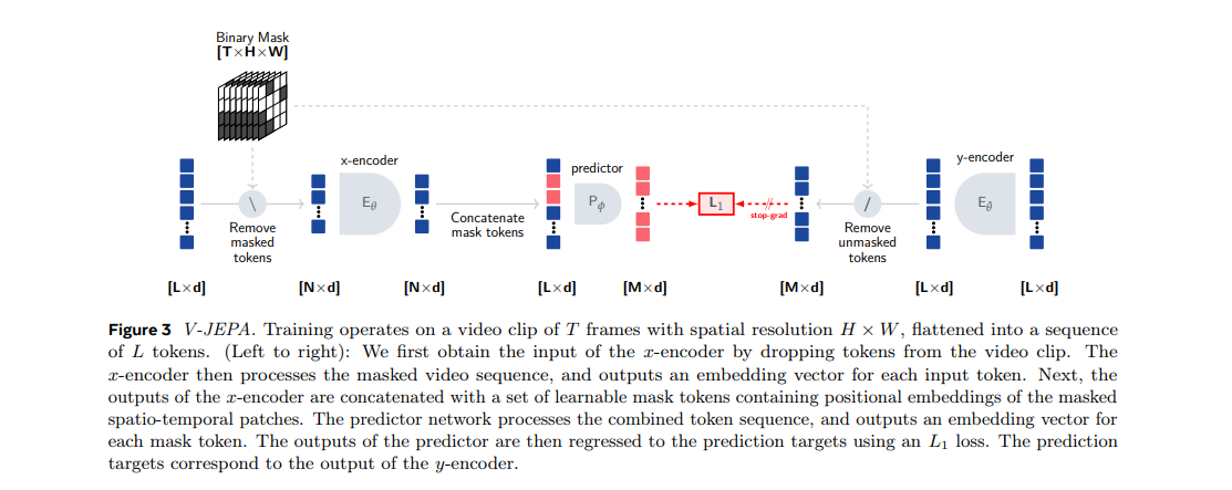
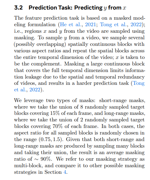
Next, certain portions are masked out. The first step is to divide the video into patches. Once that is done, it's simply a matter of unrolling it from its original 16x16x2 dimensionality. Next, they aggregate the 2D data over time, unroll it into a series of tokens, and tackle it like a language problem. They purposely mask continuous blocks in the videos to make the problem more challenging, as random masking would make it too easy to predict the content. With only the unmasked data retained, they then encode the series to create an encoded sequence.

There is a mistake in the presentation regarding the size of the patches. Each token has 512 dimensions. And at one point, they mention it's roughly 384, although that's unclear. Disregard this as it's likely just a sloppy discrepancy in the writing.

https://youtu.be/7UkJPwz_N_0?t=1820

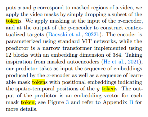
Essentially, we end up with a series of latent encodings from the unmasked parts of the video. We then fill in masked tokens for the regions we want to predict. Each of these blue squares passes through an attention mechanism. Although these tokens can contain global information, they still correspond to a given unmasked patch in the original video. We will insert tokens for the masked parts of the video. These will initially have learned mask embeddings and some positional encodings. The predictor will then predict the y embeddings, with information from both the mask tokens and the delta y.

If understood correctly, the delta y is contained within the mask token, along with information about the regions we want to predict compared to the known regions. The predictor has access to the information from x (the blue stuff) and the delta y (the red stuff). It then attempts to predict s of y. We'll take the same video and run it through the y encoder, which is an exponentially moving average of this information. We'll encode all tokens resulting in what they term 'contextualized targets'. This means each aspect can attend to every other aspect. These are the actual embeddings you'd get if you embedded the entire data point. After encoding, you mask this part and must also apply the anti-mask so you retain all the masked content. These are the targets, with the red squares specifying the parts to predict. It then predicts those roles. An L1 loss is then applied and we train and backpropagate through the predictor to the encoder via an exponentially moving average.

The overall masking ratio they referenced is 90%, meaning only about 10% of the video is X. Each spatial-temporal patch, referred to as tokens, is generated by splitting the video clip into a 3D grid consisting of 16 by 16 pixel blocks spanning two consecutive frames. The architecture includes two different networks: the encoder, which is a vision transformer serving as a video backbone. The predictor is a narrow transformer implemented using 12 blocks with an embedding dimension of 384.

Results and Evaluation | 0:42:00-10:10:10

https://youtu.be/7UkJPwz_N_0?t=2480

By the way, contrary to most large companies, Meta actually releases comprehensive tables with all the hyperparameter numbers in the appendix. This deserves a big compliment to the researchers as this paper could conceivably be reproduced.

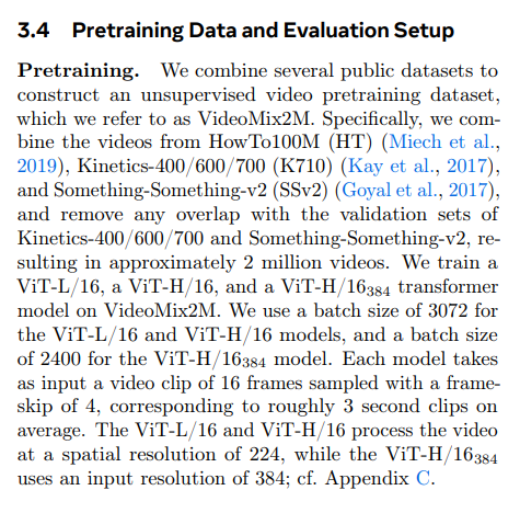
They describe the data used, the hyperparameters, and the model architecture, omitting only the exact hidden dimension. However, I suspect they retained the hidden dimension specified by VIT_H and VIT_L. Therefore, this is hypothetically reproducible, barring hardware requirements. They mention the requirement of 180 gigabytes, but it's unclear whether they meant one 180GB unit or many. Regardless, some calculations suggest they used at least 16 such units. Although, with some offloading, it may be possible to reduce this requirement. In any case, they do operate with relatively high batch sizes. High batch sizes will likely contribute to smoothing out gradients in these unsupervised representation learning methods without negatives, although this may not always be desirable. Interestingly, they mention each model takes as input a video clip of 16 frames, sampled with a frame skip of 4, approximating three-second clips. This amounts to around 1,500 patches in one data point, with a batch consisting of either 2,400 or 3,072 data points depending on the model. So, it may seem vast, but it is manageable.

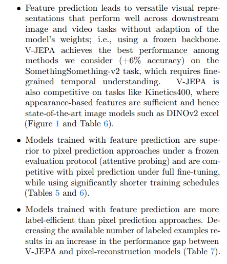
The comparative study reveals that predicting in feature space outperforms pixel space prediction in both frozen evaluation and end-to-end fine-tuning. Models predicting hidden representations perform better for downstream tasks than those predicting pixels. The evaluation involves using the pre-trained encoder for these tasks. Several data mixing and masking strategies were explored, and some showed promising results. Despite the increased workload, the method achieves similar conclusions to other models in numerous tasks, while simultaneously reducing the required sample size.

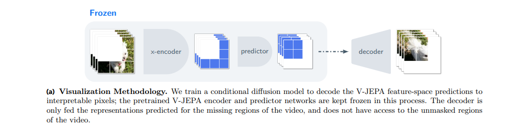
This model emphasizes qualitative assessment of the features derived by the encoder through a feature prediction objective. The decoder is trained to reconstruct the original video pixels from the predicted latent representation of masked video parts. The process involves pre-training the encoder, freezing it, and then training the decoder. The decoder solely uses the predicted latent representation of the masked region to reconstruct the pixels and does not use surrounding data. The decoded images show a good match with the original video content, although minor boundary artifacts were anticipated. This approach, known as VJEPA, is seen as a promising vector in unsupervised learning. The paper includes an extensive appendix for further information. Overall, the model's performance is commended, and the necessity of understanding the principles behind unsupervised learning is underscored.